Engineers typically design structures considering unidirectional earthquake forces. However, real earthquakes cause ground shaking which subjects structures to ground accelerations in two horizontal directions in addition to vertical acceleration. Although, building codes generally allow for the seismic design of buildings in one direction, requiring the consideration of two directions only under some circumstances, engineers are becoming more aware of situations where the consideration of two earthquake components is critical for the adequate design of a structure. One way to gain a better understanding of bidirectional response of structures is to analyze a simple pendulum system under ground accelerations in two orthogonal directions. The displacement response of such a pendulum is an orbit in a horizontal plane, whose shape depends on the nature and magnitude of the earthquake and on the relative amplitude of the ground accelerations in the two directions. Other response quantities such as the velocity and acceleration of the mass, in addition to forces such as structural, damping and inertia forces also exhibit similar bidirectional interaction. The peak of each response quantity does not necessarily occur in either of the two principal directions, but will occur at a random angle in the plane (Figure 18), and hence will be referred to as the 2D resultant. Bispec’s animation window provides several animated plots that enable a better understanding of bidirectional response (Figure 19). In addition, the model testing interactive dialog can be used to interactively examine the hysteretic response and interaction of the bidirectional hysteretic models.

Bispec computes the peak resultant by searching for the maximum value of the biaxial resultant over the analysis duration. Note that the result is different, and more accurate, than computing the SRSS of the two peaks in the two directions, which is sometimes used as an approximation, or upper limit.

For example, the peak biaxial resultant for a bidirectional displacement history (Figure 18) is computed by taking the largest mangnitude (norm) of the vector connecting the origin to point (d1,d2) in the XY plane, over the duration of the record, where d1 and d2 represent the displacement along the x and y axes:

Other spectral resultants are computed similarly. Back to the example in Figure 18, the peak displacements in the d1 and d2 directions are Sd1=5.53cm and Sd2=7.17cm, while the maximum 2D resultant is Sd2D=7.90cm. Note that since the peak d1 and d2 displacements do not generally occur at the same time, hence:

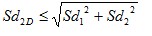
Note that in the above case: 7.90cm < (5.532+7.172)1/2 = 9.05cm

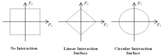
The equations governing the response of the bidirectional pendulum are similar to Equation 1. However, a system of two equations needs to be solved for the two directions. The equations may or may not be coupled. The coupling usually occurs in nonlinear systems in which the capacities in the one direction is dependent on the deformation in the other direction. Common examples of such bidirectional capacity interaction include linear and curve shaped diagrams such as those shown in Figure 20, which shows three different interaction models: no interaction (rectangular shape), linear interaction (diamond shape), and quadratic interaction (ellipse shape). See the description of the Bilinear Plasticity Model with Bidirectional Coupling.

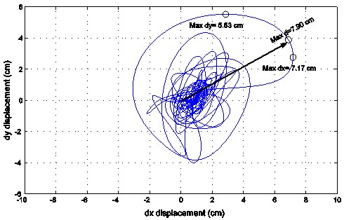
Figure 18: Bidirectional displacement interaction of a nonlinear system with a period of 0.45 seconds subjected to two ground motion components of the Northridge Rinaldi record.

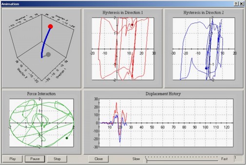
Figure 19: Bispec animation window for a nonlinear system with coupled bidirectional capacity interaction subjected to two components of the Landers earthquake.

Figure 20: Bidirectional capacity interaction models